As-Projective-As-Possible Image Stitching with Moving DLT

Julio Zaragoza*, Tat-Jun Chin*, Michael Brown and David Suter

*Corresponding authors

Quick links: Papers - Source codes - Datasets

Abstract

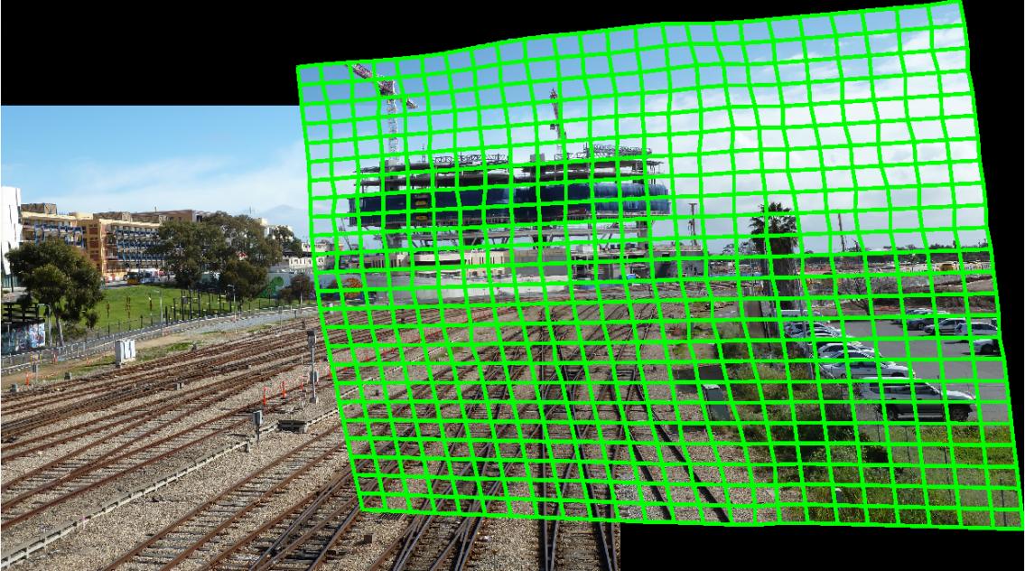
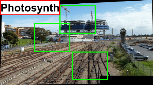
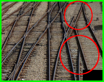
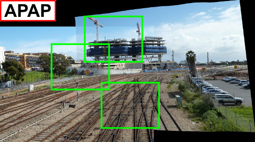
We investigate projective estimation under model inadequacies, i.e., when the underpinning assumptions of the projective model are not fully satisfied by the data. We focus on the task of image stitching which is customarily solved by estimating a projective warp - a model that is justified when the scene is planar or when the views differ purely by rotation. Such conditions are easily violated in practice, and this yields stitching results with ghosting artefacts that necessitate the usage of deghosting algorithms. To this end we propose as-projective-as-possible (APAP) warps, i.e., warps that aim to be globally projective, yet allow local non-projective deviations to account for violations to the assumed imaging conditions.

Based on a novel estimation technique called Moving Direct Linear Transformation (Moving DLT), our method seamlessly bridges image regions that are inconsistent with the projective model; see Figure 1. The result is highly accurate image stitching, with significantly reduced ghosting effects, thus lowering the dependency on post hoc deghosting.

Papers

• As-projective-as-possible Image Stitching with Moving DLT,
  Julio Zaragoza, Tat-Jun Chin, Quoc-Huy Tran, Michael Brown and David Suter,
  IEEE Transactions on Pattern Analysis and Machine Intelligence (TPAMI), 36(7):1285-1298, July 2014.
  [Paper]-[Supplementary material]-[bib]
  
  
• As-projective-as-possible Image Stitching with Moving DLT,
  Julio Zaragoza, Tat-Jun Chin, Michael Brown and David Suter,
  In Proc. IEEE Conf. on Computer Vision and Pattern Recognition (CVPR), Portland, Oregon, USA, 2013.
  [Paper]-[Supplementary material]-[bib]
  

Source codes

• [MDLT code]
  Stitches two overlapping images using an APAP warp estimated using Moving DLT (essentially this is the code for the CVPR 2013 paper).
  
  
• [BAMDLT code]
  Stitches multiple overlapping images using multiple APAP warps estimated using Bundled Moving DLT (essentially this is the code for the TPAMI 2014 paper).
  Compatibility: The code was tested with MATLAB 2013 and 2014. MATLAB 2015 changed its pooling functions, so you may have to change the code if you receive an error message when running in MATLAB 2015.
  Dependencies: You will need to install EIGEN and Google's Ceres solver and link them to your MATLAB command line when you build the corresponding MEX files.

*Kindly cite one of the above papes if using our code in your work.

Results

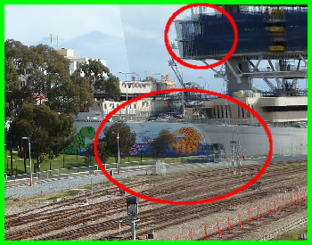
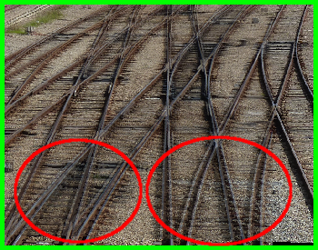
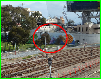
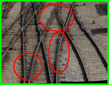
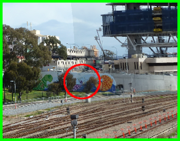
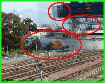
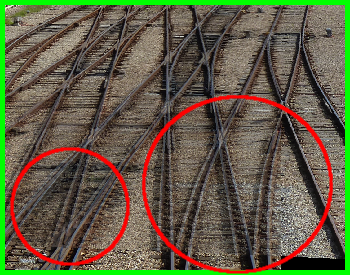
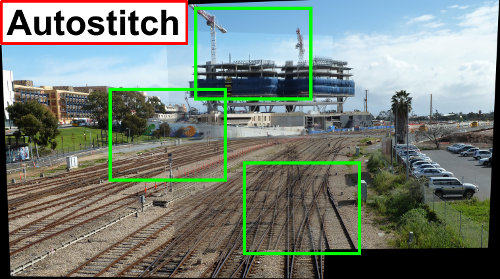
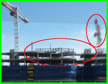
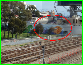
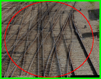
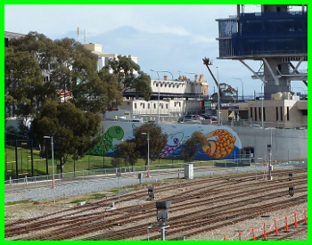
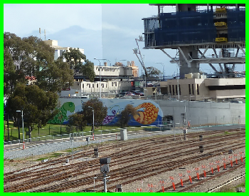
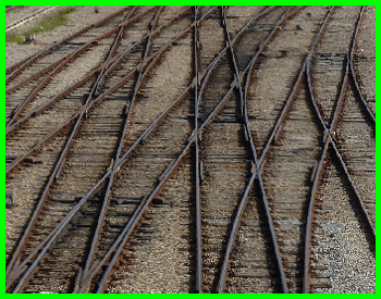
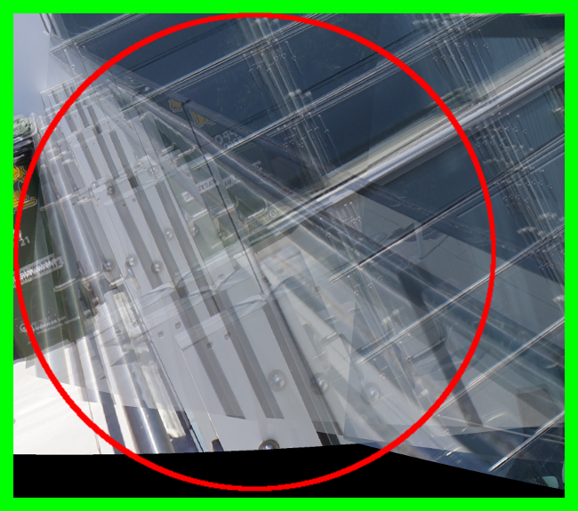
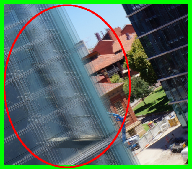
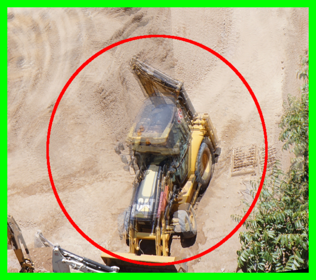
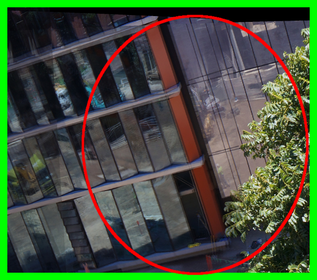
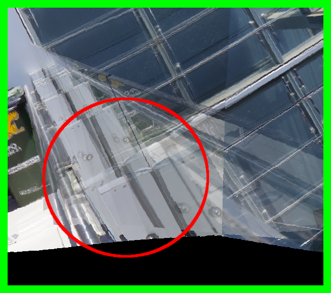
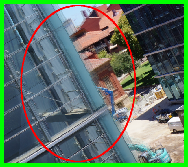
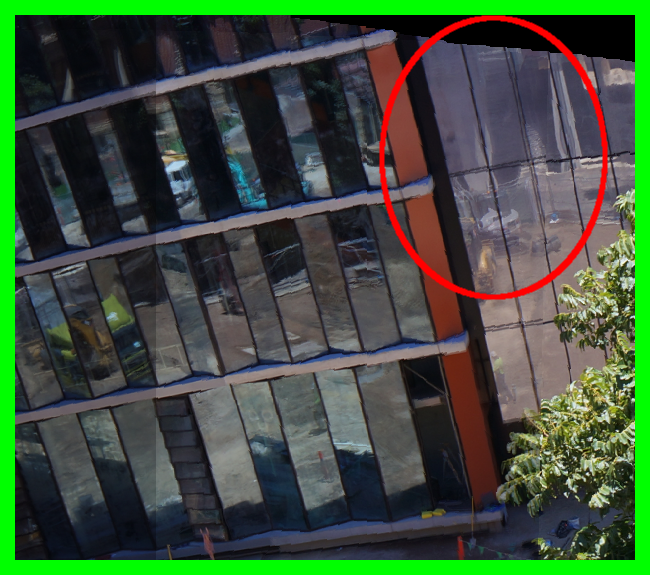
Pairwise stitching - see papers and supp materials above for more results

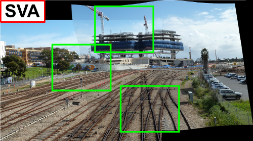
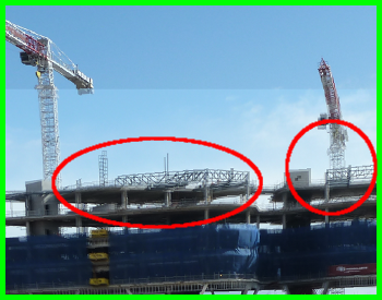
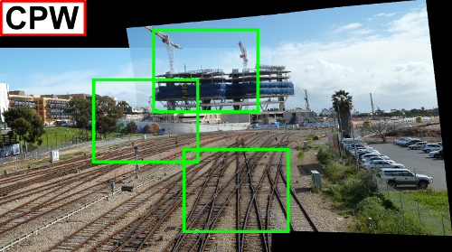
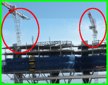
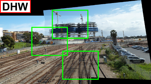
Panoramic stitching - see papers and supp materials above for more results

Evaluation data

• Dataset 1
• Dataset 2
• Dataset 3

*Kindly cite one of the above papers if using Dataset 1 in your work.

Runtime and memory consumption statistics

Processing pipeline of our MDLT code (pairwise stitching without bundle adjustment):

1. Read pair of images to stitch (image I and image I').
2. Obtain SIFT keypoint matches between I and I'.
3. Remove incorrect keypoint matches (outliers) by means on RANSAC.
4. Obtain matrix A from the set of N correct keypoint matches ({x_i,x_i'} for i=1,…,N) after RANSAC.
5. Generate mesh (of size C1 x C2) over image I.
6. (perform Moving DLT) For each vertex x* on the mesh:
1. Obtain matrix W* which contains the weights between x* and all x_i for i=1,…,N.
2. Perform SVD on matrix repmat(W*,1,9).*A.
3. Obtain homography H* from the least significant right singular vector of W*A.
7. Composite the images:
1. Obtain offset between I' and warped I.
2. Make "blank" canvas (the canvas will contain image I' and the warped image I).
3. Copy I' to the canvas in the position determined by the offset.
4. For each pixel coordinate p in image I, obtain the nearest mesh vertex x*.
1. Use the homography H* from the nearest x* to warp p in I to p' in I'.
2. Obtain the average of the intensity of pixels I(p) and I'(p').
3. Put averaged pixel in canvas (in coordinate p' + offset).

On step 6(b) of the pseudo-code, the size of matrix A is 2N x 9 and the size of W* is 2N x 1, the ".*" operator means element-wise multiplication and repmat is MATLAB's replicate and tile array function.

In the following sections we present the running time and the memory consumption statistics of our implementation of the previous pseudo-code.

Runtime statistics

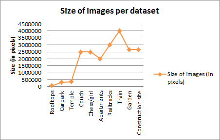
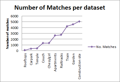
The following plots present the size of the images (in pixels) and the number of positive keypoint matches (inliers after RANSAC) per image pair (the stitching results for each one of these image pairs are available above.

The runtime of most of the image stitching methods increases with the number of keypoint matches. However, even when the number of keypoint matches is high our method is able to stitch images in reasonable time (less than 7 seconds in our experiments) as shown in the next figure.

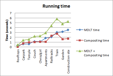
Note that the time shown in the previous plot (the green line) includes the As-Projective-As-Possible warp estimation time and the Compositing time (which includes image warping and image average blending).

As can be seen from the previous plot, the warp estimation time increases with the number of keypoint matches and the compositing time increases with the size of the images. However, our As-Projective-As-Possible image stitching method is able to maintain low running times even with large images (> 2000 x 1500 pixels) that contain thousands of keypoint matches (> 5000).

These running times were obtained on a PC with an Intel i7 950@3.07Ghz CPU and 12GB of RAM running windows 8 (64 bits).

Memory consumption

Our method requires of two main matrices for operating, namely the matrix A and the matrix W* (please refer to the paper for details). The size of these matrices depends on the number of positive keypoint matches (inliers). The following table shows the number N of positive keypoint matches per image pair and the size of the A and W* matrices. The size of the matrix A is 2N x 9 and the size of W* is 2N x 1.

The number of required Megabytes consists of the number of Megabytes required for the matrix A + number of megabytes for the matrix W* (assuming 8 bytes per entry in the matrices).

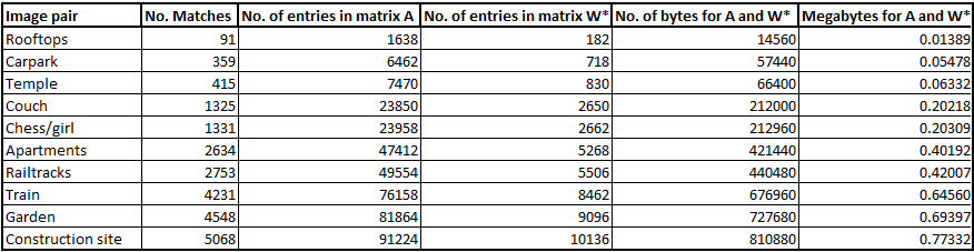
As can be seen, our method does not make use of a large amount of memory. These statistics assume that the weights for each one of the cells (W*) are obtained before performing SVD on repmat(W*,1,9).*A and then disregarded after use (i.e., disregarded after SVD on repmat(W*,1,9).*A).

EOF